distancecurrent = distanceprevious + velocityprevious * timestep
which we are trying to reconcile with a more general equation \[ x_k = a x_{k-1} \] Fortunately for us, mathematicians long ago devised “one weird trick” for representing both kinds of equations in the same way. The trick is to think of a situation (like the state of a system) not as a single number, but rather as a list of numbers called a vector, which is like a column in an Excel spreadsheet. The size of the vector (number of elements) corresponds to the number of things we want to encode about the state. For distance and velocity, we have two items in our vector: \[ x_k \equiv \begin{bmatrix} distance_k \\ velocity_k \end{bmatrix} \] Here I've used the “triple equal $\equiv$ to indicate that this is a definition: the current state is defined as a vector containing the current distance and current velocity.
So how does this help us? Well, another thing we get from linear algebra is a matrix. If a vector
is like a column of values in a spreadsheet, then a matrix is like a whole spreadsheet, or table of values.
When we multiply a matrix by a vector we get another vector of the same size:
\[
\begin{bmatrix}
a & b \\
c & d
\end{bmatrix}
\begin{bmatrix}
x \\
y
\end{bmatrix}
=
\begin{bmatrix}
ax + by \\
cx + dy
\end{bmatrix}
\]
For example:
\[
\begin{bmatrix}
8 & 3 \\
4 & 7
\end{bmatrix}
\begin{bmatrix}
2 \\
5
\end{bmatrix}
=
\begin{bmatrix}
31 \\
43
\end{bmatrix}
\]
The vectors and matrices can be of any size, as long as they match:
\[
\begin{bmatrix}
a & b & c\\
d & e & f\\
g & h & i
\end{bmatrix}
\begin{bmatrix}
x \\
y \\
z
\end{bmatrix}
=
\begin{bmatrix}
ax + by + cz\\
dx + ey + fz\\
gx + hy + iz
\end{bmatrix}
\]
We can also multiply two matrices together to get another matrix:
\[
\begin{bmatrix}
a & b & c\\
d & e & f\\
g & h & i
\end{bmatrix}
\begin{bmatrix}
r & s & t \\
u & v & w \\
x & y & z
\end{bmatrix}
=
\begin{bmatrix}
ar+bu+cx & as+bv+cy & at+bw+cz\\
dr+eu+fx & ds+ev+fy & dt+ew+fz\\
gr+hu+ix & gs+hv+iy & gt+hw+iz\\
\end{bmatrix}
\]
Adding two matrices is simpler; we just add each pair of elements:
\[
\begin{bmatrix}
a & b & c\\
d & e & f\\
g & h & i
\end{bmatrix}
+
\begin{bmatrix}
r & s & t \\
u & v & w \\
x & y & z
\end{bmatrix}
=
\begin{bmatrix}
a+r & b+s & c+t\\
d+u & e+v & f+w\\
g+x & h+y & i+z
\end{bmatrix}
\]
Returning to the task at hand, we define a matrix
\[
A =
\begin{bmatrix}
1 & timestep\\
0 & 1
\end{bmatrix}
\]
following the convention of using an uppercase letter to represent a matrix. Then our general equation is
pretty much the same:
\[ x_k = A x_{k-1} \]
which works out as we want:
\[
\begin{bmatrix}
distance_k\\
velocity_k
\end{bmatrix}
=
\begin{bmatrix}
1 & timestep\\
0 & 1
\end{bmatrix}
\begin{bmatrix}
distance_{k-1}\\
velocity_{k-1}
\end{bmatrix}
\]
\[
=
\begin{bmatrix}
1 * distance_{k-1} + timestep * velocity_{k-1}\\
0 * distance_{k-1} + 1 * velocity_{k-1}\\
\end{bmatrix}
\]
\[
=
\begin{bmatrix}
distance_{k-1} + timestep * velocity_{k-1}\\
velocity_{k-1}\\
\end{bmatrix}
\]
In other words, the current distance is the previous distance plus the previous velocity times the timestep, and
the current velocity is the same as the previous velocity. If we want to model a system in which
the velocity changes over time, we can easily modify our vector and matrix to include acceleration:
[12]
\[
\begin{bmatrix}
distance_k\\
velocity_k\\
acceleration_k
\end{bmatrix}
=
\begin{bmatrix}
1 & timestep & 0\\
0 & 1 & timestep \\
0 & 0 & 1
\end{bmatrix}
\begin{bmatrix}
distance_{k-1}\\
velocity_{k-1}\\
acceleration_{k-1}
\end{bmatrix}
\]
Previous: Adding Velocity to the System Next: Prediction and Update Revisited
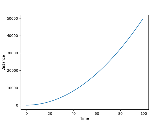
[12] Several people have emailed me to ask why the upper-right value in this matrix is 0, rather than the $0.5t^2$ value that we learned in high-school physics. The answer is that this system does not relate distance directly to acceleration; instead, it uses acceleration to update velocity, and velocity to update distance. If you're still not convinced, you can run this little Python program, which produces the expected parabolic distance curve under constant acceleration.